The IRR Trap: Why Tax Credits Break Traditional Project Finance Metrics
Investment Tax Credits (ITCs) are a powerful incentive for clean energy projects. But when tax credits exceed your equity investment, traditional IRR analysis can produce misleading results. This post uses a real battery storage (BESS) financial model to illustrate the problem and present better alternatives.
Case Study: A 100 MW / 400 MWh BESS in PJM
Consider a utility-scale battery storage project with the following structure:
| Parameter | Value |
|---|---|
| Capacity | 100 MW / 400 MWh |
| Total CAPEX | $150 million |
| Debt (80%) | $120 million at 10% over 15 years |
| Equity (20%) | $30 million |
| ITC (30%) | $45 million face value |
| ITC Cash (sold at 90%) | $40.5 million in Year 1 |
| Target Equity IRR | 12% |
Revenue Streams
| Revenue Stream | Annual Value | Calculation |
|---|---|---|
| Capacity Revenue | $7.3M | 100 MW × 60% ELCC × $333/MW-day × 365 days |
| Regulation Revenue | $8.8M | 100 MW × $20/MW-hr × 4,380 hrs (50% acceptance rate) |
| Arbitrage Revenue | ~$2.3M | 200 MWh/day × $32.01 spread × 365 days (at break-even) |
Notes:
- ELCC (Effective Load Carrying Capability) of 60% reflects PJM's capacity credit for 4-hour storage
- Regulation participation assumes 50% acceptance rate by PJM for Real-Time regulation services, with remaining time available for energy arbitrage (~200 MWh/day equivalent)
- Arbitrage revenue is the optimization variable — the model finds the minimum spread needed to achieve the target equity IRR
Regulatory Context: OBBBA (July 2025)
The One Big Beautiful Bill Act (OBBBA), signed July 4, 2025, made significant changes to clean energy tax credits. Key implications for standalone BESS:
| Item | Status Under OBBBA |
|---|---|
| ITC Availability | 30% ITC preserved for projects beginning construction through 2033 |
| Phase-out | Unlike solar/wind, standalone storage is NOT subject to the 2027 placed-in-service deadline |
| Phase-down | 25% reduction for projects beginning construction in 2034; phased out after 2035 |
| FEOC Restrictions | New Foreign Entity of Concern rules may deny credits for projects using Chinese battery components |
| Domestic Content | 40% threshold for projects begun before June 16, 2025; 45%+ after |
| Depreciation | Post-2024 construction removed from 5-year MACRS class, but 100% bonus depreciation available if placed in service after Jan 19, 2025 |
Tax Features
| Feature | Description |
|---|---|
| ITC Transferability | Post-IRA Section 6418 allows credit sales at ~90% of face value |
| NOL Carry-forwards | Tax losses in early years offset taxes in later profitable years (80% limit per TCJA/OBBBA) |
| Section 163(j) | Business interest deduction limited to 30% of ATI (EBITDA for post-2024) |
| DSCR Constraint | Optional lender requirement for debt service coverage |
Note on ITC Monetization: While Section 6418 transferability was preserved under OBBBA, new "Material Assistance" provisions add compliance hurdles for projects with certain supply chains. For projects using FEOC-affiliated components, traditional tax equity partnerships may offer more flexibility than direct credit transfers. The model assumes a clean Section 6418 transfer at 90% discount; actual market rates may vary based on supply chain and compliance factors.
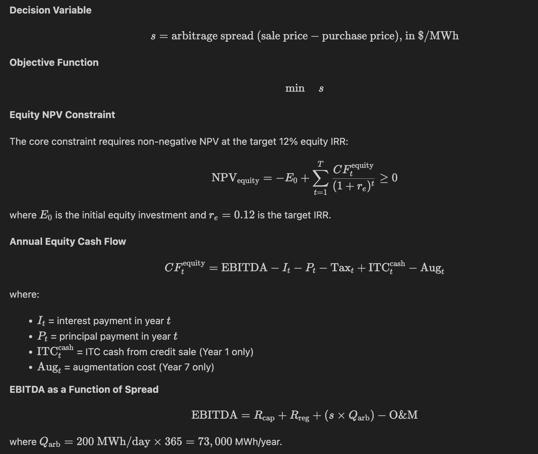
The Optimization Model
The minimum arbitrage spread that achieves the target equity IRR can be calculated using a Mixed-Integer Linear Programming (MILP) model. The integer variables are required to correctly track Net Operating Loss (NOL) carry-forwards across years.
The Cash Flow Pattern That Breaks IRR
When we run the optimization with a properly formulated model (including Section 163(j) interest limitations), we get a break-even spread of $32.3/MWh. Examining the resulting equity cash flows reveals an unusual pattern:
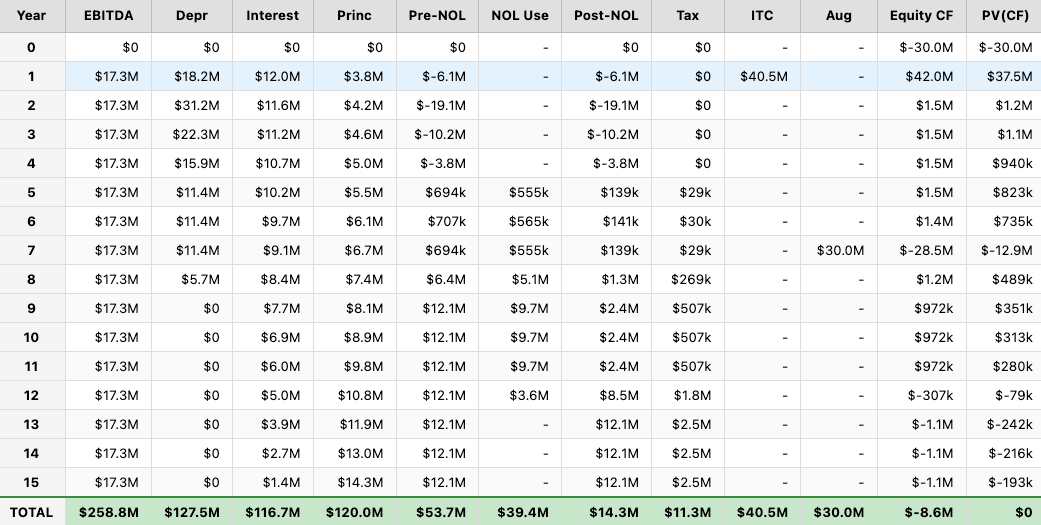
The critical observation: In Year 1, the project receives $42.0 million in cash (including $40.5M ITC cash) against a $30 million equity investment. This significant positive cash flow in Year 1 is what creates the unusual pattern that breaks traditional IRR analysis.
The IRR Calculation Problem
A fundamental assumption of IRR is that cash flows change sign only once: negative (investment) followed by positive (returns). When cash flows change sign multiple times, the IRR equation can have multiple solutions—or no real solution at all.
Our project has four sign changes:
Year 0:  Negative (equity out)
Year 1:  Positive (ITC in)       ← Sign change #1
Year 7:  Negative (augmentation) ← Sign change #2
Year 8:  Positive (operations)   ← Sign change #3
Year 12: Negative (tax payments) ← Sign change #4
By Descartes' Rule of Signs, this polynomial can have up to four real roots. When we calculate the NPV at various discount rates, we see the problem clearly:
| Discount Rate | NPV |
|---|---|
| 0% | -$8.5M |
| 5% | -$3.2M |
| 10% | -$0.4M |
| 12% | ~$0.0M |
| 15% | +$0.9M |
| 20% | +$1.3M |
Notice the inverted NPV profile: NPV increases with higher discount rates rather than decreasing. This counterintuitive behavior occurs because the large positive cash flow in Year 1 ($42M) dominates early, while the negative cash flows in later years (Years 12-15) are discounted more heavily at higher rates. At 12%, the NPV crosses zero—achieving the target IRR. But the unusual cash flow pattern still makes IRR interpretation problematic.
Three Ways to Evaluate Project Returns
- Internal Rate of Return (IRR)

Definition: The discount rate that makes NPV equal to zero.
Pros:
- Intuitive "percentage return" interpretation
- Easy to compare across projects of similar structure
- Widely understood in finance
Cons:
- Assumes reinvestment at the IRR itself (often unrealistic)
- Multiple solutions possible with non-conventional cash flows
- Meaningless when Year 1 inflows exceed the initial investment
- Can be manipulated by timing of cash flows
When to use: Single-sign-change cash flows, comparing similar projects, quick screening.
- Modified Internal Rate of Return (MIRR)

Definition: A modified IRR that assumes reinvestment at a specified "reinvestment rate" and financing at a "finance rate."
Where:
- Positive cash flows are compounded forward to Year n at the reinvestment rate
- Negative cash flows are discounted back to Year 0 at the finance rate
Pros:
- Always produces a single, unique solution
- More realistic reinvestment assumption
- Handles multiple sign changes correctly
- Less susceptible to timing manipulation
Cons:
- Requires specifying reinvestment and finance rates (adds assumptions)
- Less intuitive than IRR
- Less widely used, may require explanation to stakeholders
When to use: Projects with tax credits, interim capital expenditures, or any non-conventional cash flow pattern.
- Net Present Value (NPV) at a Fixed Discount Rate

Definition: The sum of all discounted cash flows using a predetermined hurdle rate.
Pros:
- Always produces a single, clear answer
- Directly measures value creation in dollars
- No ambiguity about reinvestment rates
- Easy to aggregate across projects (NPVs are additive)
Cons:
- Requires choosing a discount rate upfront
- Doesn't provide a "rate of return" for comparison
- Absolute dollar amount depends on project size
When to use: Comparing mutually exclusive projects, capital budgeting decisions, projects with known cost of capital.
Calculating MIRR for Our BESS Project
Let's apply MIRR to our battery project using:
- Reinvestment rate: 8% (a reasonable corporate bond rate)
- Finance rate: 10% (the project's debt rate)
import numpy_financial as npf

# Cash flows at optimal $32.29/MWh spread
cash_flows = [
    -30.0,                                 # Year 0: Equity investment
    42.0,                                  # Year 1: ITC cash + operations
    1.48, 1.48, 1.48, 1.45, 1.45,          # Years 2-6
    -28.55,                                # Year 7: Augmentation
    1.21, 0.97, 0.97, 0.97, -0.31, -1.06, -1.06,  # Years 8-14
    -1.06                                  # Year 15: Final year
]

mirr = npf.mirr(cash_flows, finance_rate=0.10, reinvest_rate=0.08)
print(f"MIRR: {mirr:.2%}")  # Output: MIRR: ~8.1%
Recommendations for BESS Project Analysis
1. Always Plot the NPV Profile
Before reporting an IRR, plot NPV against discount rate. If the curve crosses zero multiple times, or never crosses zero in a reasonable range, IRR is not a reliable metric.
2. Use MIRR for Tax Credit Projects
Any project where ITC or PTC cash flows are significant relative to equity should use MIRR instead of IRR. This includes:
- Standalone battery storage
- Solar + storage projects
- Wind projects with transferable credits
3. Be Explicit About Reinvestment Assumptions
When presenting MIRR, clearly state the reinvestment and finance rates used. A sensitivity table showing MIRR across different rate assumptions adds credibility.
| Reinvestment Rate | MIRR |
|---|---|
| 6% | 6.3% |
| 8% | 8.1% |
| 10% | 9.9% |
4. Consider NPV for Go/No-Go Decisions
For final investment decisions, NPV at the weighted average cost of capital (WACC) provides the clearest answer: "Does this project create value?" A positive NPV means yes; negative means no.
5. Verify Model Outputs Independently
When using financial models or optimization tools, always verify the solution by:
- Reconstructing cash flows manually in a spreadsheet
- Calculating NPV and IRR independently
- Checking that key constraints (like NOL utilization) behave as expected
Conclusion
The combination of large upfront tax credits, leveraged capital structures, and Section 163(j) interest limitations creates cash flow patterns that break traditional IRR analysis. In our BESS example:
- The break-even spread of $32.3/MWh achieves exactly 12% equity IRR
- Section 163(j) limits interest deductions to 30% of EBITDA (~$5.2M/year vs ~$12M scheduled in Year 1)
- TCJA/OBBBA 80% NOL limit restricts NOL usage to 80% of taxable income per year
- MIRR of ~8.1% provides a more realistic and unambiguous return measure (notably lower than the 12% IRR due to realistic reinvestment assumptions)
For clean energy project finance in the post-IRA era, where tax credit monetization is common, practitioners should:
- Default to MIRR or NPV instead of IRR
- Always visualize the NPV profile before reporting returns
- Validate financial model outputs with independent calculations
The tax incentives that make these projects economically attractive also make them analytically tricky. Understanding these nuances—and using properly formulated optimization models—separates good project finance from spreadsheet theater.
All calculations assume the post-OBBBA tax environment with 30% ITC, credit transferability, and Section 163(j) interest limitations (30% of EBITDA for post-2024 tax years).